Machine Learning

  • Ahoy there!

    Well hello. My name’s Yazin and I’m a regular guy just like you. I’ve dabbled with a bit of code in the past, namely Ruby and PHP, but I wouldn’t consider myself an expert.

    Lately, I’ve been hearing alot about Machine Learning, and I was intrigued. One thing that I found especially interesting was Tensorflow, the Machine Learning brain that Google had open sourced just last week!

    This was it .. I wanted to know more. However, there’s a ton of material out there on Machine Learning, and the topic can seem abit intimidating (especially with all the weird looking math functions).

    I heard that the best way to learn was to teach, so I’ll be documenting everything I learn here. If I don’t understand something, I’ll just say so – instead of attempting to BS my way through.

    So that’s it, I hope you’ll join me for the journey!

  • First Post! The Types of Machine Learning

    Here’s what I learned today:

    • There are a bunch of different types of Machine Learning.
    • A general impression of what can (and can’t) be achieved using Machine Learning.

    Types of Machine Learning

    There are two main types of Machine Learning:

    1. Supervised
    2. Unsupervised

    You kinda get a general sense for what these two categories might entail, but let’s talk about them abit more.

    1. Supervised Machine Learning

    In supervised learning, we are given a data set and already know what our correct output should look like .. this usually means we have some sort of hunch about the relationship between the input and the output.

    The Supervised category is further divided into 2 subcategories:

    • Regression problems: it’s where we are trying to map the inputs to a continuous output .. with infinite possible values. (Example: trying to predict the price of a stock based on historical performance of that stock)
    • Classification problems: this is where the output we’re trying to predict has a bunch of possible values, and our job is to figure out which category it falls under. (Example: given a cute picture of a kittie, trying to figure out which species it belongs to)

    2. Unsupervised Machine Learning

    Unsupervised learning, on the other hand, allows us to approach problems with little or no idea what our results should look like. We can derive structure from data where we don’t necessarily know the effect of the variables.

    We can derive this structure by clustering the data based on relationships among the variables in the data.

    With unsupervised learning there is no feedback based on the prediction results, i.e., there is no teacher to correct you. It’s not just about clustering. For example, associative memory is unsupervised learning.

    There are a bunch of categories of unsupervised machine learning:

    • Associative: Take a collection of 1000 essays written on the US Economy, and find a way to automatically group these essays into a small number that are somehow similar or related by different variables, such as word frequency, sentence length, page count, and so on.
    • Clustering: Suppose a doctor over years of experience forms associations in his mind between patient characteristics and illnesses that they have. If a new patient shows up then based on this patient’s characteristics such as symptoms, family medical history, physical attributes, mental outlook, etc the doctor associates possible illness or illnesses based on what the doctor has seen before with similar patients. This is not the same as rule based reasoning as in expert systems. In this case we would like to estimate a mapping function from patient characteristics into illnesses.
  • Some Basic definitions

    Here’s what I learned today:

    • The goal of supervised Machine Learning is to try to make good guesses, given the output of many previous guesses.
    • How to translate problems from plains words to some juicy mathematics (oh joy!).

    Goal of supervised Machine Learning

    Apparently, the entire purpose of supervised Machine Learning is to try and predict an output given (one or more) inputs.

    Some definitions

    In the examples I followed, Andrew took the case of housing prices. His imaginary friend, James, wanted to sell his house and came to Andrew asking for advice. What he then did was look at a bunch of different factors (e.g size of the house) and the impact this had on the price of the house.

    There’s a couple of important definitions to note here:

    1. The price of the house (what we’re trying to estimate) is called the output, referred to by the symbol (y) (I can now write fancy math symbols, thanks to Mr.Gaston Sanchez’s post )
    2. The inputs that influence the price of the house (or that we think influence it anyway) are called .. well, inputs. The symbol for those is \(x\) (and potentially, \(x_1\), \(x_2\), …).
    3. Our goal, in a supervised learning scenario is to come up with some sort of relationship (equation, not that other type you silly person) between the input(s) and the output. We’d then be able to use that relationship to predict the \(y\) from the \(x\)’s. This relationship is called a hypothesis, and is referenced by the symbol \(h\).

    Let’s talk abit more about point #3 above, about the hypothesis \(h\). Essentially, if the relationship is linear (Andrew promises to tell us later how to get the best possible fit, linear or otherwise), then the relationship takes the form of:

    \[h = \theta_0 + \theta_1 x\]

    This looks kinda similar to an equation I remember from school:

    \[y = mx + c \text{ (or } y = c + mx)\]

    That’s the straight line formula, where \(m\) is the gradient/slope, \(c\) is the y-intercept and \(x, y\) are both coordinates of any point on the line. It’s clear, just by comparing the two, that \(\theta_0 = c\) (the y-intercept) and \(\theta_1 = m\) (the gradient/slope). In general, we call these \(\theta\) things parameters of the hypothesis (so we don’t have to call them theta things the whole time).

    The bottom line is this: if we know (or can somehow calculate) what the parameters (\(\theta_0, \theta_1\)) are, then we can predict the values of \(y\) given \(x\).. all without even needing a crystal ball!

    For our purposes, we’re not supposed to dig too deep into this just yet. Things get icky pretty quickly when you add multiple \(x\)’s, and higher order hypotheses (like quadratic equations, cubic equations, etc.).

    Let’s not worry about all that just yet .. and focus on getting this darn thing to work with the most basic case first.

    Training data

    Like we said earlier, we’ll be given a bunch of training data (which are really just \((x, y)\) pairs .. and later asked to predict the value of \(y\) when given \(x\).

    Here’s what a sample training data set might look like:

    Size in ft2 Price (x $1,000)
    2104 460
    1416 232
    1534 315

    The total number of rows (or pairs) of training data is called \(m\), and we’ll be using that a bunch of times in our calculations.

    Now, our job, as mentioned earlier is to find a relationship that connects our features (\(x\)’s) to our predicted value of \(y\).

    We’ve now got a bunch of points, and we’re trying to predict the \(y\) value given an \(x\) .. you can probably already see where this is going .. we need to find the line of best fit.

    Finding the line of best fit

    Calculating the line of best fit is pretty easy to do, visually (see my hand-drawn masterpiece below).

    Line of best fit

    When you try to do it in math though, the equations can end up looking pretty scary. The concept however is a simple one.

    To get the line of best fit, you first need to define what “fit” means .. in our case, this means calculating some sort of figure that allows you to differentiate a “good” fit from a bad one.

    We call this the cost function. To find the cost of a particular hypothesis, all you really have to do is calculate how often the hypothesis is able to predict the output correctly. If all the predictions are 100% spot-on, then it has a cost of zero. If the predictions are crap, it’ll have a high cost. Bottom line is, we’re trying to optimize for cost – the lower, the better.

    Here’s how we can calculate the cost:

    1. For each point in our training dataset, we find the “distance” between the predicted output (i.e. our hypothesis \(h\)) and the actual output (\(y\)).
    2. We then square this distance, to get rid of weird stuff that happens with negative points (an error is an error, whether the distance is positive or negative).
    3. Let’s now add all of those squares up.
    4. Finally take the average of all those figures, so that we can compare errors across different datasets (regardless of the number of data points in any particular set).
    5. This final step is purely for convenience, and involves multiplying the end result by \(\frac12\) .. to make calculations on the derivative “cleaner” (since \( \frac12 \times 2 = 1 \))

    Here’s how that looks like mathematically (brace yourselves):

    \[J(\theta_0, \theta_1) = \frac{1}{2m} \sum_{i=1}^m \left( h(x^{(i)}) - y^{(i)} \right)^2\]

    I’m not entirely sure why the cost function uses the symbol \(J\) (I would’ve personally used the symbol \(C\), since you know, it’s a Cost function .. but maybe it was already taken or something).

  • Gradient Descent

    So now we have a hypothesis function and we’ve got a way to measure how accurate it is. All we need now is a way to improve our hypothesis function, eventually finding the best possible \(\theta_0, \theta_1\) values (that minimize our cost).

    That’s where gradient descent comes in.

    Imagine plotting our \(\theta_0, \theta_1\) parameters on the \(x, y\) axes .. and a 3 dimensional \(y\) axis showing the corresponding cost function \(J(\theta_0, \theta_1)\) for those \(\theta_1, \theta_1\) values.

    Here’s what that would look like:

    Cost function vs thetas

    What we’re looking for is the point on the graph would the lowest cost, which would represent the pit in the center. That’s the sweet spot.. and the values of \(\theta_0\) and \(\theta_1\) at that point are what we are looking for (to optimize our holy hypothesis function \(h\)).

    Since plotting these pretty graphs is not always possible (imagine what it would look like if you had just 20 features instead of 1).

    Instead then, what we need to do is find a mathematical way to get the answers we need.

    The Concept

    At the core of the gradient descent technique is a very simple idea. If we can take a starting point - any starting point - and then take a tiny step “downhill” (towards a point with a lower cost), then we’ll eventually get to a pit .. somewhere where we can’t descend any further without going back up. This point is known as the local minima and that’s what we’re aiming for.

    The only question is: “how do we know which way is downhill?”.

    Well, that’s where your old from high school - derivatives - come in. If you remember one thing about derivatives in school, it’s that a derivative is the slope at a given point (if you’re completely lost, check out this excellent introduction to derivates).

    So all we need to do then is follow the derivative (the slope at a particular point), and it will give us a direction to move towards.

    \[\theta_j := \theta_j - \alpha[\text{derivative of J}]\] \[\theta_j := \theta_j - \alpha \frac{\partial}{\partial \theta_j} J(\theta_0, \theta_1)\]

    Gradient Descent for Linear Regression

    Assuming we’ve only got one \(x\) and one \(y\) (carrying on the example from the last post), we can start substituting equations in to really drive this point home.

    Let’s start by substituting for the value of \(J\) which we derived in the previous post as:

    \[J(\theta_0, \theta_1) = \frac{1}{2m} \sum_{i=1}^m \left( h(x^{(i)}) - y^{(i)} \right)^2\]

    .. this results in:

    \[\theta_j := \theta_j - \alpha \frac{\partial}{\partial \theta_j} \left( \frac{1}{2m} \sum_{i=1}^m \left( h(x^{(i)}) - y^{(i)} \right)^2 \right)\]

    Since we have two variables that we’re trying to optimize (namely \(\theta_0)\) and \(\theta_1\)), we have to use what’s known in the geeky world of mathematics as partial derivatives. While it may sound like I just turned all Math professor on you, it’s actually a simple concept.

    It’s like a normal derivative, where you treat everything as a constant except the variable you are deriving by. If that’s not enough by way of introduction, check this great explanation on the Math StackExchange site.

    Ok, so here are the final equations we’re looking for (in their simplified form, after rearranging and stuff):

    \[\begin{align} \theta_0 & := \theta_0 - \alpha \frac{1}{m} \sum_{i=1}^m \left(\theta_0 + \theta_{1}x^{(i)} - y^{(i)}\right) \\ \theta_1 & := \theta_1 - \alpha \frac{1}{m} \sum_{i=1}^m \left(\theta_0 + \theta_{1}x^{(i)} - y^{(i)}\right) x^{(i)} \end{align}\]

    She’s a real beauty, ain’t she?

    And this is just one step. We’ll be running this calculation many, many times .. as we journey down the hill of cost, to the local minima (sometimes thousands of times even).

    The code

    Nothing drives a point home like seeing some code, and I really struggled to get my head around this whole vector business until I actually saw it implemented in traditional arrays.

    from numpy import *
    
    # y = theta_1 * x + theta_0
    # Not actually required in the gradient descent calculation; just used to verify
    # the sanity of the results :)
    def compute_error_for_line_given_points(theta_0, theta_1, points):
      totalError = 0
      for i in range(0, len(points)):
          x = points[i, 0]
          y = points[i, 1]
          totalError += (y - (theta_1 * x + theta_0)) ** 2
      return totalError / (2 * float(len(points)))
    
    def step_gradient(theta_0_current, theta_1_current, points, alpha):
      # Gets called for each iteration of 'alpha'
      theta_0_gradient = 0
      theta_1_gradient = 0
      m = float(len(points))
      for i in range(0, len(points)):
        x = points[i, 0]
        y = points[i, 1]
        theta_0_gradient += -(1/m) * (y - ((theta_1_current * x) + theta_0_current))
        theta_1_gradient += -(1/m) * x * (y - ((theta_1_current * x) + theta_0_current))
      new_theta_0 = theta_0_current - (alpha * theta_0_gradient)
      new_theta_1 = theta_1_current - (alpha * theta_1_gradient)
      return [new_theta_0, new_theta_1]
    
    def gradient_descent_runner(points, starting_theta_0, starting_theta_1, alpha, num_iterations):
      # This method simply runs the 'step_gradient' method num_iterations times,
      # updating the values of theta_0, theta_1 after each iteration.
      theta_0 = starting_theta_0
      theta_1 = starting_theta_1
      for i in range(num_iterations):
        theta_0, theta_1 = step_gradient(theta_0, theta_1, array(points), alpha)
      return [theta_0, theta_1]
    
    def run():
      # This method reads all of our data points (x, y)'s and calls the
      # 'gradient_descent_runner' passing in all of the variables
      points = genfromtxt("data.csv", delimiter=",")
      alpha = 0.0001
      initial_theta_0 = 0 # initial y-intercept guess
      initial_theta_1 = 0 # initial slope guess
      num_iterations = 1000
      print "Starting gradient descent at theta_0 = {0}, theta_1 = {1}, error = {2}".format(initial_theta_0, initial_theta_1, compute_error_for_line_given_points(initial_theta_0, initial_theta_1, points))
      print "Running..."
      [theta_0, theta_1] = gradient_descent_runner(points, initial_theta_0, initial_theta_1, alpha, num_iterations)
      print "After {0} iterations theta_0 = {1}, theta_1 = {2}, error = {3}".format(num_iterations, theta_0, theta_1, compute_error_for_line_given_points(theta_0, theta_1, points))
    
    if __name__ == '__main__':
      run()

    You’ll find the data.csv file here.

    Here’s what the output looks like:

    > $python gradient_descent_example.py
    Starting gradient descent at theta_0 = 0, theta_1 = 0, error = 2782.55391724
    Running...
    After 1000 iterations theta_0 = 0.0590585566422, theta_1 = 1.47833132745, error = 56.3163353936

    It took me a while to wrap my head around this, and to get the code to a working state. Matt Nedrich’s post on the topic was very helpful.

    Note: I’ve used Python in the example above, but going forward most examples will be written using Octave.

  • Multivariate Linear Regression

    Here’s the deal. So far, we’d only discussed the most basic possible example: a case where you had:

    • a single feature (our \(x\), the area of the house)
    • a single output (our \(y\), the price of the house)
    • and a linear relationship between the two

    Now, we’re about to grow up .. because in the real world, we don’t just have a single feature. We have many .. sometimes even thousands!

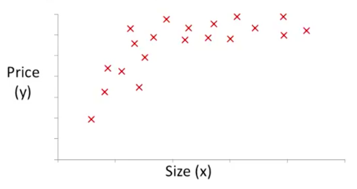
    Think about it .. it sounds absolutely absurd that you would even think that it’s possible to accurately predict the price of a house based on area alone! So many other things matter, like the number of rooms, the floors, the size of the garden, how old it is and it’s sentimental value to you (actually, scratch that last one).

    So that’s what we’ll be covering in this post .. how to consider a more complex prediction example.

    Don’t forget our goal .. we’re still trying to come up with a hypothesis function that would allow us to accurately predict the price of the house, based on the inputs we’re given.

    Let’s do this.

    Revisiting our (now broken) equations

    We’re going to have to go back and fix the equations we discussed earlier. The definitions (or rather, the meaning) of the equations won’t change .. but we no longer have just one \(x\) to deal with.

    First, a few new definitions.

    Since we have many \(x\)’s now, let’s give them subscripts (e.g. \(x_1, x_2, x_3\)) to refer to our different features.

    Note that we already said that the bracketed-superscripts for \(x\) (like \(x^{(1)}, x^{(2)}\), etc.) represent samples in the training set. This still holds true. We just have to get used to seeing things like \(x_1^{(2)}\), which is the second row (or data point in our training data) of the first feature.

    We also need a way to refer to the total number of features we’ve got .. let’s go ahead and call that \(n\).

    Now that we have that out of the way, let’s take a look at those equations .. starting with our hypothesis \(h_0(x)\).

    Hypothesis function \(h_\theta(x)\)

    Before (we had only one \(x\)): \(h_\theta(x) = \theta_0 + \theta_1 x\)

    After (we have many \(x\)’s): \(h_\theta(x) = \theta_0 + \theta_1 x_1 + \theta_2 x_2 + \text{...}\)

    You’ll notice something going on here .. all the terms have both \(\theta\)’s and \(x\)’s .. except for that first one, the lonely looking \(\theta_0\). To simplify things, let’s go ahead and give it an \(x_0\) that has a value of 1 (so that it doesn’t change the equation in any way).

    Now, it looks like:

    \(h_\theta(x) = \theta_0 x_0 + \theta_1 x_1 + \theta_2 x_2 + \text{...}\) (where \(x_0=1\))

    Let’s take the next jump .. let’s lump up all of those \(\theta_0, \theta_1, \theta_2\), … parameters into a single vector like so:

    \[\theta = \begin{bmatrix} \theta_0 \\ \theta_1 \\ \theta_2 \\ \vdots \\ \theta_n \end{bmatrix}\]

    .. and similarly ..

    \[x = \begin{bmatrix} x_0 \\ x_1 \\ x_2 \\ \vdots \\ x_n \end{bmatrix}\]

    Those weird looking towers are known in the mathematics parlance as matrices. If you have no idea what those are, you can think of them as layers of numbers, not very different from your good ole’ Big Mac. If you want to learn more, just check out this video here. You may or may not remember that a matrix with just one column is known as a vector.

    So here, we’re treating our \(\theta\) and our \(x\) as a single vector, as opposed to many tiny numbers with little subscripts.

    So now, our new hypothesis equation will simply be:

    \[h_\theta(x) = \theta^T x\]

    That weird looking T on top of the \(\theta\) is known as the transpose of \(\theta\), or \(\theta\) flipped on it’s side like so:

    \[\theta^T = \begin{bmatrix} \theta_0 & \theta_1 & \theta_2 & \cdots & \theta_n \end{bmatrix}\]

    The reason we use \(\theta^T\) and not \(\theta\) is so that the multiplication will work (if you don’t know how to multiply matrices, check out this short video for a primer).

    We now have a new equation for our hypothesis function! (keeping in mind that \(x_0=1\) or this whole business just won’t work).

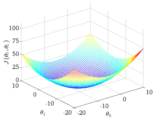
    Cost function \(J(\theta)\)

    Our new and improved cost function now looks like this:

    \[J(\theta) = \frac{1}{2m} \sum_{i=1}^m \left(\ h_\theta(x^{(i)}) - y^{(i)} \right)^2\]

    Next, let’s take a look at our gradient descent equation.

    Gradient descent

    If you’ll recall, the gradient descent equation in the case of a single feature looked like this:

    \[\theta_j := \theta_j - \alpha \frac{\partial}{\partial \theta_j} J(\theta)\]

    Substituting for \(J(\theta)\), that becomes:

    \[\theta_j := \theta_j - \alpha \frac{\partial}{\partial \theta_j} \left( \frac{1}{2m} \sum_{i=1}^m \left( h(x^{(i)}) - y^{(i)} \right)^2 \right)\]

    We then computed the partial derivative for each of our \(\theta_0, \theta_1\) individually, resulting in:

    \[\begin{align} \theta_0 & := \theta_0 - \alpha \frac{1}{m} \sum_{i=1}^m \left(h(x^{(i)}) - y^{(i)}\right) \\ \theta_1 & := \theta_1 - \alpha \frac{1}{m} \sum_{i=1}^m \left(h(x^{(i)}) - y^{(i)}\right) x^{(i)} \end{align}\]

    When replacing this with multiple features, my expectation was that things would get ickier .. much ickier. In fact, I was pleasantly surprised to realize that it wasn’t the case at all.

    A fundamental property of partial derivatives is that you only calculate the derivative with reference to the variable you’re deriving with (which are our \(\theta_0, \theta_1\), etc. variables).

    Since we’re only going to be computing the derivative with respect to one of these variables at a time, the resulting derivative looks just like the \(\theta_1\) term above.

    Namely, it’ll be:

    \[\begin{align} \theta_0 & := \theta_0 - \alpha \frac{1}{m} \sum_{i=1}^m \left(h(x^{(i)}) - y^{(i)}\right) \\ \theta_1 & := \theta_1 - \alpha \frac{1}{m} \sum_{i=1}^m \left(h(x^{(i)}) - y^{(i)}\right) x_1^{(i)} \\ \theta_2 & := \theta_2 - \alpha \frac{1}{m} \sum_{i=1}^m \left(h(x^{(i)}) - y^{(i)}\right) x_2^{(i)} \end{align}\]

    Not too bad, huh?

    All the equations look similar except for the first one. Wait .. remember that lonely \(x_0=1\) we were talking about earlier? Well, turns out it’s their in that first equation .. but we just didn’t see it (since it’s equal to 1):

    \[\theta_0 := \theta_0 - \alpha \frac{1}{m} \sum_{i=1}^m \left(h(x^{(i)}) - y^{(i)}\right) x_0^{(i)}\]

    Now let’s write it in the general form:

    \[\theta_j := \theta_j - \alpha \frac{1}{m} \sum_{i=1}^m \left(h(x^{(i)}) - y^{(i)}\right) x_j^{(i)}\]

    Kill the feature subset (represented by the subscript \(j\), since \(\theta\) is a vector anyway) and we’re left with:

    \[\theta := \theta - \alpha \frac{1}{m} \sum_{i=1}^m \left(h(x^{(i)}) - y^{(i)}\right) x^{(i)}\]

    I don’t know about you but I’m feeling like I’ve had my fair share of math for now .. let’s jump into some good ole’ fashioned code.

    Implementing things in code

    Alright, enough of this math business .. let’s take a look at some code. I’ll be using Octave in this example, since that’s what the Machine Learning course uses (and it makes dealing with matrices, as well as all the rest of the Machine Learning stuff pretty easy).

    So yeah, Octave. The syntax is pretty self-explanatory, though writing it will take a bit of getting used to (at least for me anyway).

  • Tricks to make Gradient Descent converge faster

    Trick #1: Normalize your data

    You know how you were always trying to fit in as a kid? Well, it turns out that’s good advice for our features to heed.

    It can be proved that if your features have greatly varying ranges, then it would almost certainly take longer for gradient descent to find the local minima.

    For example, let’s take the features below:

    \(x_1\) = Size of the bedroom (0 - 2000 ft\(^2\))

    \(x_2\) = Number of bedrooms (1 - 5 rooms)

    The ideal feature would fit within the range \(-1 \le x \le +1\)

    Just keep in mind that this is an approximate range ( \(-2 \le x \le 3 \) is fine too .. but \(-1,000 \le x \le 250\) is not)

    Knowing what we know now, we can easily normalize \(x_1, x_2\) to fit within that range by doing:

    \[x_1 = \frac{\text{Size of bedroom}}{2000}\] \[x_2 = \frac{\text{Number of bedrooms}}{5}\]

    Voila, we’re all done.

    Note: There’s another form of normalization called “Mean normalization” where you try to center the averages. Frankly, I’m feeling way too lazy to be writing about that right now .. so we’re skipping it. Read about it here if you dig that sort of thing.

    Trick #2: Picking a learning rate, \(\alpha\)

    We’ve discussed \(\alpha\) before, but we haven’t really talked much about how we initially decide on what value to choose.

    Turns out, you just gotta try a bunch of values and see what works best. Rather than brute forcing every number in existence though, you can take a more visual approach.

    Try to plot number of iterations vs. \(J(\theta)\):

    Number of iterations vs. Cost

    If your \(J(\theta)\) isn’t decreasing after every iteration, then something isn’t right.

    You can try the following values for \(\alpha\), starting with the smallest and moving up (until you see the values diverge):

    0.001, 0.003, 0.01, 0.03, 0.1, 0.3, 1 (so basically just start at 0.001 and keep multiplying by approx. 3)

    Interesting Note

    An interesting aside is that you can make all sorts of crazy changes to your initial data and magically conjure new features that way.

    The action starts with a plot of the feature itself vs. the output you’re measuring:

    Fitting a curve

    Looking at this curve, you might think .. you know what? There kinda looks like there might be some square-root relationship going on between the \(x\) and the \(y\) .. so why don’t I just use \(\sqrt(x)\) as a feature instead of plain old \(x\) (or even in addition to the \(x\)).

    That’s totally cool. Now, you’re hypothesis would look like:

    \[h(\theta) = \theta_0 + \theta_1 x + \theta_2 \sqrt{x}\]

subscribe via RSS